Project Overview: I analyzed the CDC’s Behavioral Risk Factor Surveillance System (BRFSS) 2015 dataset using K-means clustering to identify groups based on reported health and life satisfaction patterns. By combining health indicators with socioeconomic factors (household income and education) I aimed to understand how these social determinants relate to individual health outcomes. The initial dataset contained over 400,000 observations, which I reduced to 15,032 by cleaning out incomplete data.
Variables Used:
- General Health (GENHLTH): Measures perceived overall health (higher values indicate poorer health).
- Mental Health (MENTHLTH): Number of days mental health negatively impacted daily life (higher values indicate more frequent struggles).
- Physical Health (PHYSHLTH): Number of days physical health was poor.
- Life Satisfaction (LSATISFY): Reflects self-reported quality of life (higher values mean lower satisfaction).
Clustering Analysis and Findings:
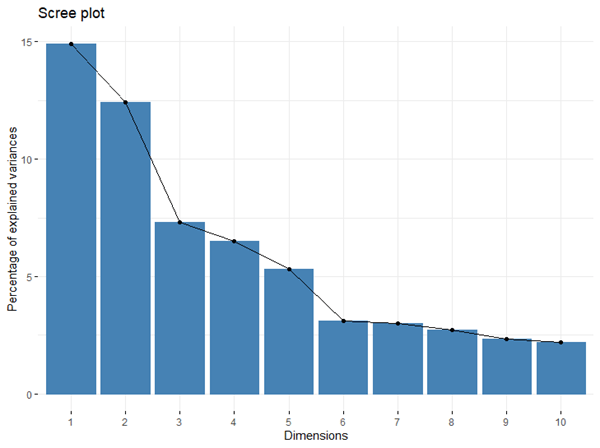
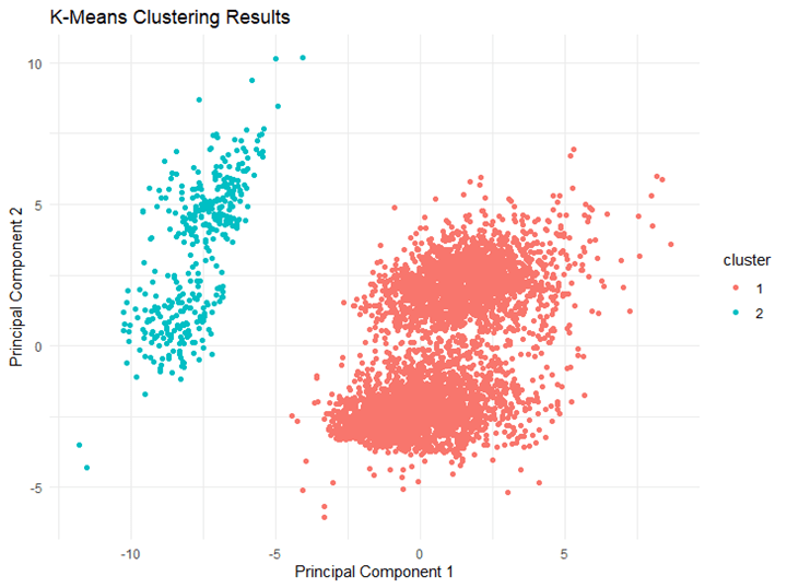
Analysis 1: Health and Income Using the elbow method, I determined an optimal cluster count of 6. Here’s what I found:
- Cluster 0 (18%): Highest income group (>$75,000) with excellent health and high life satisfaction.
- Cluster 1 (9%): Lowest income group ($10,000-$15,000) with significant health challenges but moderate life satisfaction.
- Cluster 2 (6%): Middle-income earners ($35,000-$50,000) with the poorest health indicators but moderate satisfaction.
- Cluster 3 (14%): Middle-income group ($35,000-$50,000) with good health and high life satisfaction.
- Cluster 4 (35%): Largest group with highest income levels (>$75,000), showing good health and high life satisfaction.
- Cluster 5 (18%): Upper middle-income earners ($50,000-$75,000) with similar good health and high satisfaction.
This analysis highlights that higher income is associated with better health outcomes and life satisfaction, reinforcing existing evidence on the impact of socioeconomic factors.

Analysis 2: Health and Education For this analysis, I used 9 clusters based on the elbow method. Key findings include:
- Cluster 0 (19%): Highly educated (college graduates) with very good health and high life satisfaction.
- Cluster 2 (4%): Individuals with some college education but severe physical and mental health challenges.
- Cluster 6 (8%): High school graduates with moderate health challenges yet high life satisfaction, suggesting resilience.
- Other clusters demonstrated how different levels of educational attainment impact health outcomes and satisfaction levels.

Key Takeaways:
- The majority of the dataset reported moderate to high life satisfaction. Clusters with the highest educational levels (college graduates) were concentrated in groups with higher satisfaction and better health outcomes.
- Cluster 2 showed the widest spread of life satisfaction and predominantly consisted of individuals with high school education or lower, indicating the need for a more in-depth understanding of what contributes to variability in well-being among this group.
Critical Reflections and Future Directions:
- Dataset Limitations: The dataset is predominantly composed of white and highly educated individuals, limiting the generalizability of these findings. To make public health insights more inclusive, future analyses should use more diverse datasets.
- Adding More Variables: Incorporating factors like healthcare access, chronic disease indicators, and racial identity could provide a more comprehensive understanding of health disparities and social determinants.
- Methodological Improvements: While K-means clustering in Weka is effective for straightforward analysis, it has limitations with non-linear relationships and imbalanced datasets. Future projects will explore more advanced clustering techniques like DBSCAN or hierarchical clustering using Python for deeper insights.
- Actionable Steps: I plan to expand future analyses by integrating more demographic variables and advanced techniques to provide a fuller picture of factors influencing health and life satisfaction in the U.S. population.
By continually refining my approach, I aim to produce more meaningful and comprehensive public health insights. This project served as a valuable practice in understanding how socioeconomic factors impact health outcomes.
Full lab write up