Empowering Rural Communities Through Culturally Competent Health Tech

Assignment Background

For my Implementing Health Informatics Initiatives for Emerging Leaders course in the Gillings School of Global Public Health at UNC–Chapel Hill, I developed an informatics-based concept proposal for the NSF America’s Seed Fund. My proposal focuses on a mobile application designed to support multiple chronic diseases in rural communities, where health literacy tends to be lower. Below is a subsection of that proposal.

HealthBridge Rural: A Culturally Competent Health Literacy App for Chronic Disease Prevention and Management 

Introduction 

Rural communities face persistent health inequities driven by limited healthcare access, transportation barriers, low health literacy, and high prevalence of preventable chronic diseases such as diabetes, hypertension, COPD, and cardiovascular disease. According to CDC data, adults in rural areas are more likely to die prematurely from five leading causes1 and report lower rates of preventive care and health literacy2. Traditional health apps often fail to reach these communities because they assume consistent access to broadband internet, cultural familiarity with digital tools, and standardized health literacy levels. 

In these areas, cultural norms, economic hardship, and health mistrust create additional barriers. For example, a patient may understand their diagnosis but not how to modify their lifestyle affordably or safely. Information about exercise, nutrition, and stress reduction is often disconnected from local contexts; recipes may not utilize affordable, readily available foods, and exercise recommendations rarely account for environmental or safety constraints. 

HealthBridge Rural aims to close this gap by providing culturally competent, low-cost, and locally contextualized health information to empower residents to take small, achievable steps toward improved health. It combines behavioral science, public health data, and user-centered design to build trust, comprehension, and sustainable engagement across several chronic conditions. 

Application Overview: 

HealthBridge Rural is a mobile and web-based application designed using Dr. Mica Endsley’s Situation Awareness-Oriented Design (SAOD) principles—Perception, Comprehension, and Projection—to support informed, context-driven decision-making3. The app offers a personalized dashboard that integrates educational tools, behavioral nudges, and local resource directories to help users navigate their health more effectively. 

1. Perception  

 The app aggregates publicly available and user-reported data to present relevant, localized health insights: 

  • Maps of affordable grocery stores, farmers’ markets that accept EBT, community gardens, and food giveaway programs. 
  •  Maps of parks, community recreation centers, and walking trails. 
  • Listings of free or low-cost health programs, community clinics, and smoking cessation groups. 
  • Daily check-ins for sleep, stress, diet, and activity. 

2. Comprehension  

 AI translates medical information into culturally relevant, accessible language. 

 Examples: 

  • “Instead of sugary tea, try this $2 pitcher of flavored water using ingredients from Dollar General.” 
  • “Here’s how to manage stress when working long shifts—three exercises that take less than 5 minutes.” 
  • Audio and visual literacy options for users with limited reading skills. 

The AI integrates local cultural insights, such as traditional foods or family-centered values to ensure content resonates with the user’s lived experiences. 

3. Projection – Supporting Informed Action 

 Based on users’ inputs, HealthBridge Rural generates personalized recommendations and reminders: 

  • Predictive prompts (“You’ve been logging low activity—try this free walking club nearby.”) 
  • Behavior simulation (“If you switch one meal per day to a home-cooked option, here’s the 3-month health impact and savings.”) 
  • Smart notifications tailored to disease risk factors (e.g., hypertension management reminders). 

Logic Model (Adaptation of Endsley’s Situational Awareness Model): 

Level Description HealthBridge Rural Application 
Perception Awareness of environment and current state Local maps, cost-aware recipes, nearby resources 
Comprehension Understanding significance of data AI-curated education, culturally adapted health tips 
Projection Anticipating outcomes and next steps Personalized goals, predictive alerts, self-monitoring tools 

1 https://www.cdc.gov/health-equity-chronic-disease/health-equity-rural-communities/index.html 

2  https://www.ruralhealthinfo.org/toolkits/health-literacy/1/barriers 

3 Endsley, M. R., & Jones, D. G. (2024). Situation Awareness Oriented Design: Review and Future Directions. International Journal of Human–Computer Interaction, 40(7), 1487–1504. https://doi.org/10.1080/10447318.2024.2318884 

Using Machine Learning to Understand Treatment Delays in Breast Cancer Care

Introduction

Cancer treatment delays and modifications can significantly impact patient survival and quality of life. Research has consistently shown that marginalized populations, including Black, Hispanic, Asian, and American Indian/Alaska Native (AIAN) patients, experience higher rates of late-stage cancer diagnoses and lower rates of timely treatment.

For my project, I used machine learning models to examine how race, socioeconomic status, tumor characteristics, cancer stage, grade, subtype, age, clinical trial participation, and time to treatment initiation predict treatment interruptions in breast cancer patients.

This project highlights both the potential and limitations of using machine learning for predicting healthcare disparities in cancer treatment.


Dataset:

This project utilized Simulacrum v2.1.0, a synthetic dataset derived from the National Disease Registration Service (NDRS) Cancer Analysis System at NHS England. While this dataset mimics real-world cancer data, it ensures patient anonymity.

After data cleaning and removing incomplete observations, the dataset contained 69,367 patients, all diagnosed with breast cancer.

Demographics Overview

  • Gender Distribution:
    • Women: 98.7%
    • Men: 1.3% (Male breast cancer cases were retained for analysis.)
  • Age Distribution:
    • Mean Age: 61.06 years
    • Median Age: 61 years
  • Racial Distribution:
    • White: 85.9%
    • Asian: 3.7%
    • Black: 1.9%
    • Other: 1.7%
    • Mixed Race: 0.6%
    • Unknown: 6.1% (Reweighting was applied to mitigate algorithmic bias.)

  • Neighborhood Deprivation (Socioeconomic Status):
    • Scored from 1 (most deprived) to 5 (least deprived).
    • The dataset was fairly balanced across deprivation levels.

Average Time to Treatment Initiation (by Race)

  • Overall: 61 days
  • Other Racial Groups: 71 days
  • Black Patients: 63 days
  • White Patients: 62 days
  • Asian Patients: 54 days
  • Mixed Race Patients: 45 days
  • Unknown Race: 57 days

Clinical Trial Participation

  • 84.4% of patients were enrolled in a clinical trial.

Data Processing & Feature Engineering

1. Cleaning & Standardizing Data

  • Removed inconsistent staging classifications.
  • Imputed missing values for key variables such as comorbidity scores and time to treatment initiation.

2. Encoding Variables

  • One-Hot Encoding:
    • Race, tumor subtype, estrogen receptor (ER), progesterone receptor (PR), and HER2 status.
  • Ordinal Encoding:
    • Tumor stage, node stage, metastasis stage, overall stage, grade, and deprivation index.

3. Feature Engineering

  • Created a new feature,ANY_REGIMEN_MOD
    • Combined dose reduction, time delay, and early termination variables into one binary target variable.
  • Grouped tumor biomarkers into cancer subtypes:
    • Luminal A: ER+, PR+, HER2- (Least aggressive)
    • Luminal B: ER+, PR+, HER2+ (Slightly more aggressive)
    • HER2-Enriched: ER-, PR-, HER2+
    • Triple Negative (Basal-like): ER-, PR-, HER2- (Most aggressive)

Bias Mitigation Strategies

1. Gender Bias

  • While 98% of patients were female, male breast cancer cases were retained for rare case analysis.
  • Applied weighting techniques to balance gender representation during model training.

2. Racial Bias

  • Since 85% of patients in the dataset were White, inverse weighting was applied to ensure fair contributions across racial groups.

Machine Learning Models & Performance

I trained Random Forest and XGBoost models to predict treatment modifications.

1. Initial Model Performance (Random Forest & XGBoost)

Results were poor. The models performed only slightly better than random guessing.

2. Hyperparameter Tuning & Feature Selection

  • Used GridSearchCV to optimize parameters.
  • Dropped the least important features and retrained the models.
  • Results did not improve, and performance worsened in some cases.

3. Model Performance Issues

  • Models failed to generalize to testing data.
  • ROC AUC scores hovered around 0.5, meaning models were barely better than random guessing.
  • Models overfitted the ‘no treatment modification’ group, inaccurately predicting treatment delays.

4. Alternative Models Attempted

To address these issues, I tested additional models:

  • Support Vector Machines (SVM)
  • Neural Networks
  • Logistic Regression
  • K-Nearest Neighbors (KNN)
  • Naïve Bayes

Findings from Alternative Models:

  • SVM and Logistic Regression performed best (Accuracy: 0.65), but logistic regression completely failed at predicting treatment modifications.
  • Neural Networks, KNN, and Naïve Bayes were slightly better balanced but still had low accuracy (~0.60–0.62).

5. Last Attempt – Oversampling with SMOTE

  • Used Synthetic Minority Oversampling (SMOTE) to balance the dataset.
  • SVM improved slightly, but performance gains were minimal.

Uncovering Insights Through Clustering

Since predictive modeling was unsuccessful, I conducted clustering analysis to find patterns in the data.

Three Distinct Patient Clusters Emerged:

Cluster 0: Moderate-Stage Cancer (35.4% Treatment Modifications)

  • Average Age: 60.8
  • Tumor Stage: T2, N0.7, M0.03 (Localized)
  • Time to Treatment: 32.6 days

Cluster 1: Early-Stage Cancer with Delayed Treatment (36.7% Treatment Modifications)

  • Average Age: 61.0
  • Tumor Stage: T1, N0.03, M0.0 (Localized, very early-stage)
  • Time to Treatment: 46.8 days (longest)

Cluster 2: Older Patients with Shortest Time to Treatment (36.8% Treatment Modifications)

  • Average Age: 69.4 years
  • Higher Comorbidities (Charlson Score = 0.63)
  • Time to Treatment: 14.8 days (shortest)

Key Takeaways from Clustering:

  • Cluster 1 had the longest time to treatment despite being early-stage. Further investigation needed.
  • Older patients (Cluster 2) received faster treatment but had more comorbidities.

Conclusion & Next Steps

Machine learning models failed to predict treatment modifications accurately.
Clustering analysis revealed patterns in treatment delays and patient subgroups.

Future Steps:

  1. Explore more sophisticated models (Deep Learning, Bayesian Networks).
  2. Use real-world data instead of synthetic datasets.
  3. Investigate non-quantifiable factors, like patient-provider interactions and healthcare policies.

Final Thoughts

This project highlighted the complexity of predicting cancer treatment interruptions and the importance of interdisciplinary approaches in health equity research.

If you’re interested in machine learning for healthcare, data-driven health equity research, or predictive modeling, let’s connect!

Clustering Individuals Based on Health and Socioeconomic Indicators Using the CDC’s BRFSS Data

Project Overview: I analyzed the CDC’s Behavioral Risk Factor Surveillance System (BRFSS) 2015 dataset using K-means clustering to identify groups based on reported health and life satisfaction patterns. By combining health indicators with socioeconomic factors (household income and education) I aimed to understand how these social determinants relate to individual health outcomes. The initial dataset contained over 400,000 observations, which I reduced to 15,032 by cleaning out incomplete data.

Variables Used:

  • General Health (GENHLTH): Measures perceived overall health (higher values indicate poorer health).
  • Mental Health (MENTHLTH): Number of days mental health negatively impacted daily life (higher values indicate more frequent struggles).
  • Physical Health (PHYSHLTH): Number of days physical health was poor.
  • Life Satisfaction (LSATISFY): Reflects self-reported quality of life (higher values mean lower satisfaction).

Clustering Analysis and Findings:

Analysis 1: Health and Income Using the elbow method, I determined an optimal cluster count of 6. Here’s what I found:

  • Cluster 0 (18%): Highest income group (>$75,000) with excellent health and high life satisfaction.
  • Cluster 1 (9%): Lowest income group ($10,000-$15,000) with significant health challenges but moderate life satisfaction.
  • Cluster 2 (6%): Middle-income earners ($35,000-$50,000) with the poorest health indicators but moderate satisfaction.
  • Cluster 3 (14%): Middle-income group ($35,000-$50,000) with good health and high life satisfaction.
  • Cluster 4 (35%): Largest group with highest income levels (>$75,000), showing good health and high life satisfaction.
  • Cluster 5 (18%): Upper middle-income earners ($50,000-$75,000) with similar good health and high satisfaction.

This analysis highlights that higher income is associated with better health outcomes and life satisfaction, reinforcing existing evidence on the impact of socioeconomic factors.

This image displays the relationship between income (INCOME2, y-axis) and physical health (PHYSHLTH, x-axis). Clusters 0, 3, and 5 are skewed to the left, indicating that these groups experience fewer days where physical health negatively impacts their daily life. These clusters also belong to the highest income categories, suggesting that higher income groups tend to have better physical health outcomes. In contrast, Cluster 2 is skewed to the right, showing a higher number of days of poor physical health, with income levels spread throughout the range. Clusters 1 and 2 have a denser concentration of observations on the right side, reflecting the groups with the poorest health outcomes, regardless of their income distribution.

Analysis 2: Health and Education For this analysis, I used 9 clusters based on the elbow method. Key findings include:

  • Cluster 0 (19%): Highly educated (college graduates) with very good health and high life satisfaction.
  • Cluster 2 (4%): Individuals with some college education but severe physical and mental health challenges.
  • Cluster 6 (8%): High school graduates with moderate health challenges yet high life satisfaction, suggesting resilience.
  • Other clusters demonstrated how different levels of educational attainment impact health outcomes and satisfaction levels.
In general, the majority of the data set reported high or moderate life satisfaction. Clusters 0, 1, and 4 show high concentrations toward the left side of the plot, indicating high life satisfaction. These clusters also represent individuals with the highest levels of educational attainment (primarily college graduates). In contrast, Cluster 2 displays the widest spread in life satisfaction levels and consists mostly of individuals with high school education or lower.

Key Takeaways:

  • The majority of the dataset reported moderate to high life satisfaction. Clusters with the highest educational levels (college graduates) were concentrated in groups with higher satisfaction and better health outcomes.
  • Cluster 2 showed the widest spread of life satisfaction and predominantly consisted of individuals with high school education or lower, indicating the need for a more in-depth understanding of what contributes to variability in well-being among this group.

Critical Reflections and Future Directions:

  1. Dataset Limitations: The dataset is predominantly composed of white and highly educated individuals, limiting the generalizability of these findings. To make public health insights more inclusive, future analyses should use more diverse datasets.
  2. Adding More Variables: Incorporating factors like healthcare access, chronic disease indicators, and racial identity could provide a more comprehensive understanding of health disparities and social determinants.
  3. Methodological Improvements: While K-means clustering in Weka is effective for straightforward analysis, it has limitations with non-linear relationships and imbalanced datasets. Future projects will explore more advanced clustering techniques like DBSCAN or hierarchical clustering using Python for deeper insights.
  4. Actionable Steps: I plan to expand future analyses by integrating more demographic variables and advanced techniques to provide a fuller picture of factors influencing health and life satisfaction in the U.S. population.

By continually refining my approach, I aim to produce more meaningful and comprehensive public health insights. This project served as a valuable practice in understanding how socioeconomic factors impact health outcomes.

Full lab write up

Exploring Social Data with Principal Component Analysis (PCA)

During my summer internship at the NIH, I was introduced to Principal Component Analysis (PCA) through a colleague. Intrigued by PCA’s potential, I wanted to apply this technique to social data, particularly from the National Longitudinal Study of Adolescent to Adult Health (Add Health), which contains a rich dataset of 10,237 variables.

Objective

My goal was to identify underlying patterns in social factors like academic performance, self-esteem, relationships with parents, and substance use. I narrowed down the vast dataset to 50 key variables to uncover trends and relationships.

Approach

I began by learning PCA through various resources, including Kaggle tutorials and DataCamp courses. I also revisited linear algebra fundamentals to ensure a solid mathematical understanding.

For the analysis:

  1. Data Cleaning: Initially, I filled missing values with -1, but realized this approach needed refinement based on the scale of responses.
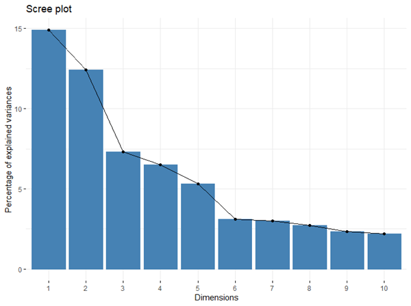
  2. PCA Implementation: I used the prcomp function in R to perform PCA. Focusing on the first two principal components, which explained 27.3% of the variance, allowed me to manage the complexity.
  3. Visualization: I created a biplot to visualize the results. Due to the large number of variables, I filtered for the most influential ones, revealing that alcohol usage significantly impacts dataset variability.

Findings

  • Principal Component 1: Associated with lower self-esteem, moderate alcohol use, and less satisfaction in parent relationships.
  • Principal Component 2: Linked to positive school behavior, higher grades, less loneliness, and lower alcohol consumption.

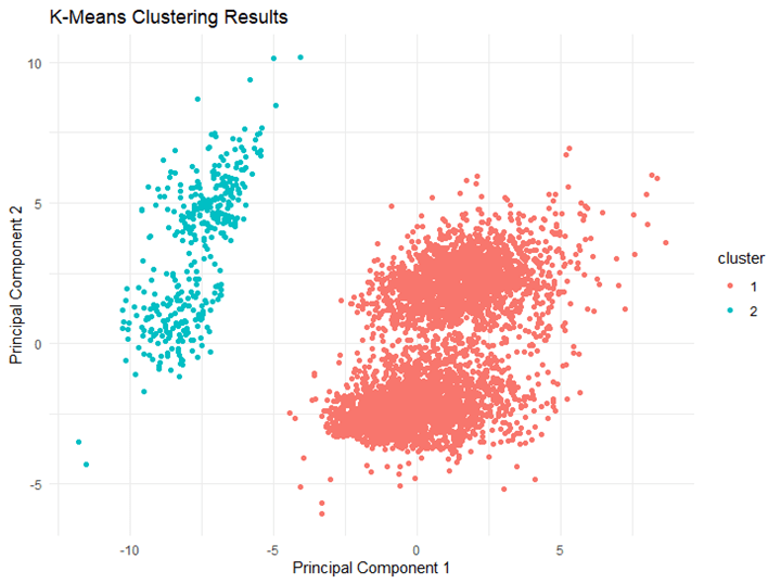
Using K-means clustering, I identified two groups:

  • Cluster 1 (Red): Higher on PC1, indicating lower self-esteem and weaker parental bonds.
  • Cluster 2 (Blue): Higher on PC2, suggesting better academic performance and less loneliness.

The analysis highlighted how alcohol usage and social factors contribute to overall data variability. I plan to refine my approach with a smaller dataset for better interpretation.

Resources Used